matrix methods
notes from linear algebra
Vectors
Canonical Unit Vectors (standard basis vectors)
\( \mathbb{e}_i\) = where the i-th position is 1 and all other positions are 0. For example, in \( \mathbb{R}^3 \): \[ \mathbf{e}_1 = (1, 0, 0), \quad \mathbf{e}_2 = (0, 1, 0), \quad \mathbf{e}_3 = (0, 0, 1) \] Any vector \( \mathbf{v} \in \mathbb{R}^n \) can be expressed as: \[ \mathbf{v} = v_1 \mathbf{e}_1 + v_2 \mathbf{e}_2 + \cdots + v_n \mathbf{e}_n \]Inner Products (dot products)
\[ a \cdot b = a^T b \] Properties:1. \( b^T a = a^T b \)
2. \( (\gamma a)^T b = \gamma (a^T b)\)
scaling a then taking dot product with b is same as taking the dot product of a and b then scaling it
3. \( (a + b)^T c = a^T c + b^T c \)
the dot product of c with the sum of a and b is the same as the dot product of (a and c) plus (b and c)
Operations:
1. Picking out the i'th element: \( \quad e_{i}^T a = a_{i} \)
2. Sum of elements: \( \quad 1_n a = a_1 + a_2 + a_3 ... a_n \)
3. Sum of squares: \( \quad a^T a = a_{1}^2 + a_{2}^2 + a_{3}^2 ... a_{n}^2 \) \( \quad \quad a^T a = 0 \quad \text{iff} \quad a = 0 \)
Tensor Product (Outer Product)
\[ \mathbf{a} \otimes \mathbf{b} = \mathbf{a} \mathbf{b}^T \] \[ a = \begin{bmatrix} a^0 \\ a^1 \\ a^2 \\ a^3 \end{bmatrix}, \quad b = \begin{bmatrix} b^0 \\ b^1 \\ b^2 \\ b^3 \end{bmatrix} \quad \quad a \otimes b = \begin{bmatrix} a^0 b^0 & a^0 b^1 & a^0 b^2 & a^0 b^3 \\ a^1 b^0 & a^1 b^1 & a^1 b^2 & a^1 b^3 \\ a^2 b^0 & a^2 b^1 & a^2 b^2 & a^2 b^3 \\ a^3 b^0 & a^3 b^1 & a^3 b^2 & a^3 b^3 \end{bmatrix} \]Linear Functions
Satisfies superposition property (both homogeneity + additivity):1. Homogeneity: \( f(ax) = a f(x) \)
2. Additivity: \( f(x + y) = f(x) + f(y) \)
Any linear function can be represented as a dot product \(f(x) = a^T x \) and any dot product function is linear (for some fixed vector a)
\[ f(c_1 x + c_2 y) = \] \[ a^T (c_1 x + c_2 y) = a^T (c_1 x) + a^T (c_2 y) = c_1(a^T x) + c_2(a^T y) \] \[ = c_1 f(x) + c_2 f(y) \]
Affine Functions
Affine functions are linear functions \( f(x) = a^T x \) but offset by some b (linear always go through (0,0), affine functions need not): \[ f(x) = a^T x + b \]Taylor Approximation
A first order taylor series is a linear approximation of the function f.Using a nearby point z, we can approximate f(x) using: \[ \hat{f}(x) = f(z) + \Delta f(z)(x - z) \]
Norm and Distance
\[ ||x|| = \sqrt{x_{1}^2 + x_{2}^2 ...} = \sqrt{x^T x} \] \[ ||x||^2 = \textbf{sum of squares} = x_{1}^2 + x_{2}^2 ... = x^T x \] Properties:1. \( ||cx|| = |c|||x|| \)
2. \( ||x + y|| \leq ||x|| + ||y|| \)
3. \( ||x|| \geq 0 \)
4. \( ||x|| = 0 \quad \) iff \( \quad x = 0 \)
Mean square value: \( \frac{||x||^2}{n} \)
Root Mean square value (RMS): \( \frac{||x||}{\sqrt{n}} \quad \) (i.e., typical value of \( |x_i| \))
Block (stacked) Vectors:
\[ ||(a,b,c)||^2 = a^T a + b^T b + c^T c = ||a||^2 + ||b||^2 + ||c||^2 \]
Chebyshev's Inequality:
- Judges the size of a vector
- Most numbers in a vector can't be much bigger than its RMS
Suppose k elements in vector x is larger than some a. Then:
- Number of elements \( |x_i| > a \) is no more than \( ||x||^2 / a^2 \)
- The percentage of elements \( |x_i| \geq a RMS(x) \) is \( \leq \frac{1}{a^2} \)
\[ \frac{||x||^2}{a^2} \geq k \quad \text{or} \quad \frac{k}{n} \leq (\frac{RMS(x)}{a})^2 \]
Distance:
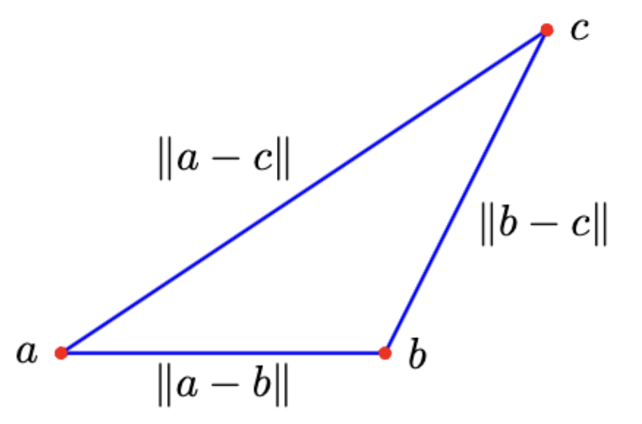
Distance between a and b is: \( || a - b || \)
Triangle Inequality: Sum of twox sides must be greater than or equal to third side
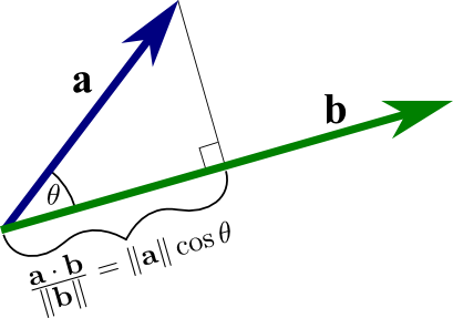
Cauchy Schwartz Inequality: \( |a \cdot b| \leq ||a||||b|| \)
Average of \( x = \frac{ x_1 + x_2 + ...}{n} = \frac{1^T x }{n} \)
Demeaned vector \( \tilde{x} = x - avg(x)1 \)
Standard deviation of \( x = rms(\tilde{x}) = \frac{||x - avg(x)1|| }{\sqrt{n}} \)
\( rms(x)^2 = avg(x)^2 + std(x)^2 \)
Standardized vector \( z = \frac{\tilde{x}}{std(x)}\)
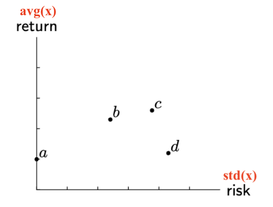
Example in Finance:
x = time series of returns
avd(x) = average return
std(x) = volatility
Risk-Reward Plot:
Angles
\[\theta = \cos^{-1}\left(\frac{\mathbf{a} \cdot \mathbf{b}}{\|\mathbf{a}\| \|\mathbf{b}\|}\right)\]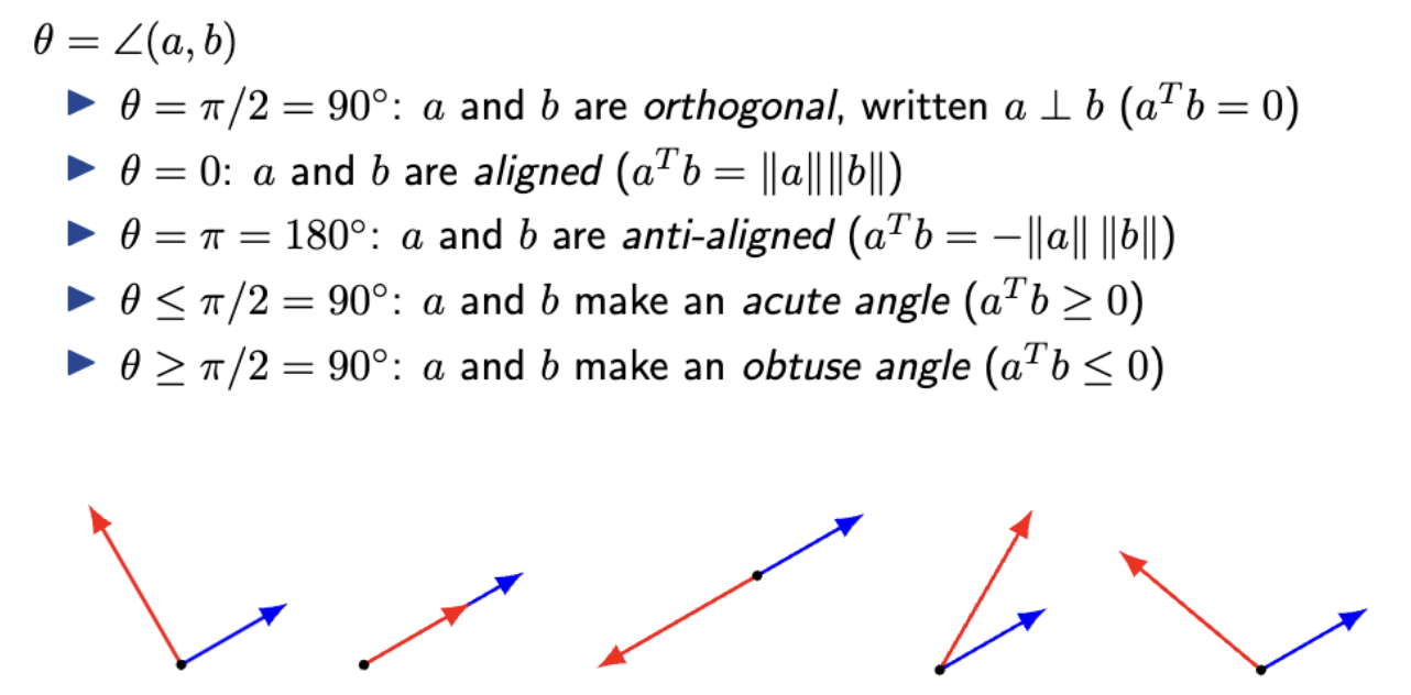
Linear Independence
Vectors \( \{\mathbf{v}_1, \mathbf{v}_2, \dots, \mathbf{v}_k\} \) are linearly independent if \( c_1, c_2, \dots, c_k \) = 0 is the ONLY solution to:
\[ c_1 \mathbf{v}_1 + c_2 \mathbf{v}_2 + \dots + c_k \mathbf{v}_k = \mathbf{0}. \]
Basis
A set of vectors \( \{\mathbf{b}_1, \mathbf{b}_2, \dots, \mathbf{b}_n\} \) forms a basis for a vector space \( V \) if:
- The vectors are linearly independent.
- The vectors span the whole space \( V \) (i.e., any vector in \( V \) can be expressed as a linear combination of the basis vectors)
Orthonormal Expansion
- Orthonormal vectors are orthogonal and its norm is 1
If \( \{\mathbf{a}_1, \mathbf{a}_2, \dots, \mathbf{a}_n\} \) is an orthonormal basis for a vector space \( V \), any vector \( \mathbf{v} \in V \) can be expressed as:
\[ \mathbf{v} = \sum_{i=1}^n (\mathbf{v} \cdot \mathbf{a}_i) \mathbf{a}_i, \]
Gram-Schmidt Process
Orthogonal vectors means they are linearly independent but linearly independent vectors DOES NOT indicate they are orthogonal
Gram-Schmidt allows us to construct an orthonormal basis from a set of linearly independent vectors
Given a set of linearly independent vectors \( \{\mathbf{v}_1, \mathbf{v}_2, \dots, \mathbf{v}_n\} \), the Gram-Schmidt process generates an orthonormal set \( \{\mathbf{u}_1, \mathbf{u}_2, \dots, \mathbf{u}_n\} \) as follows:
\[ \mathbf{u}_1 = \frac{\mathbf{v}_1}{\|\mathbf{v}_1\|} \] \[ \mathbf{u}_2 = \frac{\mathbf{v}_2 - (\mathbf{v}_2 \cdot \mathbf{u}_1) \mathbf{u}_1}{\| \mathbf{v}_2 - (\mathbf{v}_2 \cdot \mathbf{u}_1) \mathbf{u}_1 \|} \] \[ \mathbf{u}_3 = \frac{\mathbf{v}_3 - (\mathbf{v}_3 \cdot \mathbf{u}_1) \mathbf{u}_1 - (\mathbf{v}_3 \cdot \mathbf{u}_2) \mathbf{u}_2}{\| \mathbf{v}_3 - (\mathbf{v}_3 \cdot \mathbf{u}_1) \mathbf{u}_1 - (\mathbf{v}_3 \cdot \mathbf{u}_2) \mathbf{u}_2 \|} \]
This process continues for all \( \mathbf{v}_i \) to produce orthonormal vectors.
Matrices
Lower Triangular Matrices
\[ \begin{bmatrix} a_{11} & 0 & 0 & 0 \\ a_{21} & a_{22} & 0 & 0 \\ a_{31} & a_{32} & a_{33} & 0 \\ a_{41} & a_{42} & a_{43} & a_{44} \end{bmatrix} \begin{bmatrix} x_1 \\ x_2 \\ x_3 \\ x_4 \end{bmatrix} = \begin{bmatrix} a_{11}x_1 \\ a_{21}x_1 + a_{22}x_2 \\ a_{31}x_1 + a_{32}x_2 + a_{33}x_3 \\ a_{41}x_1 + a_{42}x_2 + a_{43}x_3 + a_{44}x_4 \end{bmatrix} \]Difference Matrices
\[ \begin{bmatrix} -1 & 1 & 0 & 0 \\ 0 & -1 & 1 & 0 \\ 0 & 0 & -1 & 1 \end{bmatrix} \begin{bmatrix} x_1 \\ x_2 \\ x_3 \\ x_4 \end{bmatrix} = \begin{bmatrix} x_2 - x_1 \\ x_3 - x_2 \\ x_4 - x_3 \end{bmatrix} \]Rotation Matrices
A 2D rotation matrix for an angle $\theta$ is given by: \[ R(\theta) = \begin{bmatrix} \cos\theta & -\sin\theta \\ \sin\theta & \cos\theta \end{bmatrix} \]Incidence Matrix
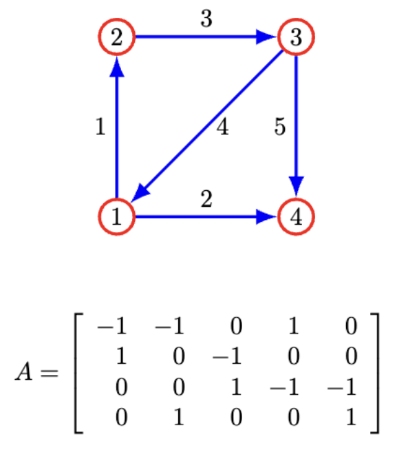
For a simple undirected graph with m edges and n nodes, the incidence matrix \( A \in \mathbb{R}^{nodes \times edges} \) is defined as: \[ A_{i,j} = \begin{cases} 1, & \text{if edge } j \text{ incoming to } i \\ -1, & \text{if edge } j \text{ leaving } i \\ 0, & \text{no connection} \end{cases} \]
Incidence Matrix
A simple example of a 1D convolution smoothing matrix with a 3-point moving average kernel is: \[ C = \begin{bmatrix} \frac{1}{3} & \frac{1}{3} & \frac{1}{3} & 0 & \dots & 0 \\ 0 & \frac{1}{3} & \frac{1}{3} & \frac{1}{3} & \dots & 0 \\ \vdots & \vdots & \vdots & \vdots & \ddots & \vdots \\ 0 & 0 & 0 & \dots & \frac{1}{3} & \frac{1}{3} & \frac{1}{3} \end{bmatrix} \]Matrix Powers and Adjacency Matrix
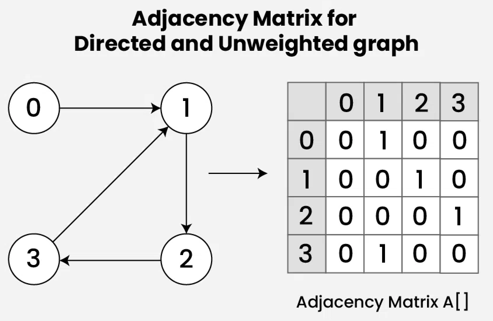
Matrix Powers: The k'th power of an adjacency matrix \( A^k \) tells us number of paths of length k between 2 vertices
- Node 0 to 2 has length 2
- The entry at (0,2) of AA = 2
Convolution Matrices
\[ c_k = \sum_{i+j=k+1} a_i b_j \] \( c_1 \) means k = 2, so compute sum of products where (i = 1, j = 1)\( c_2 \) means k = 3, so compute sum of products where (i = 1, j = 2) and (i = 2, j = 1)
\( c_2 \) means k = 4, so compute sum of products where (i = j = 2), (j = 1, i = 3), and (j = 3, i = 1)
Polynomial Multiplication
\(c_k\) gives us the coefficients in \(p(x)q(x)\) \[ p(x) = a_1 + a_2 x + a_3 x^2 + \ldots a_n x^{n-1} \quad \quad q(x) = b_1 + b_2 x + b_3 x^2 \ldots b_m x^{m-1} \] \[ p(x)q(x) = c_1 + c_2 x + c_3 x^2 + \ldots c_{n+m-1} x^{n+m-2} \]
Linear Mapping
A linear mapping \( f: \mathbb{R}^n \to \mathbb{R}^m \) can be represented by a matrix \( A_{m \times n} \) such that for any vector \( x \in \mathbb{R}^n \): \[ f(x) = Ax \] 1. f will always send 0 to 0If f(0) \( \neq \) 0, f is NOT linear
If f(0) \(=\) 0, f may or may not be linear
2. \( f(\alpha x + \beta y) = A(\alpha x + \beta y) = \alpha Ax + \beta Ay \)
3. If f does not have a matrix representation, it is NONLINEAR
Finding A Given x
For an \(n\)-vector \(\mathbf{x} = (x_1, \dots, x_n)\), we use the standard unit vectors to write: \[ \mathbf{x} = x_1 \mathbf{e}_1 + x_2 \mathbf{e}_2 + \cdots + x_n \mathbf{e}_n \] Since \(f\) is linear, we have: \[ f(\mathbf{x}) = x_1 f(\mathbf{e}_1) + x_2 f(\mathbf{e}_2) + \cdots + x_n f(\mathbf{e}_n) \] Now, we put together the \(m \times n\) matrix \(A\) column by column: \[ A = \left[ f(\mathbf{e}_1) \,\, f(\mathbf{e}_2) \,\, \cdots \,\, f(\mathbf{e}_n) \right] \] Thus, we can write: \[ f(\mathbf{x}) = x_1 f(\mathbf{e}_1) + x_2 f(\mathbf{e}_2) + \cdots + x_n f(\mathbf{e}_n) = A \begin{bmatrix} x_1 \\ x_2 \\ \vdots \\ x_n \end{bmatrix} \]Price-Demand Elasticity Model
- Prices are given by an \( n \)-vector \( p \).- Demand (e.g., units sold) is given as an \( n \)-vector \( d \).
- The fractional (percent) change in price of good \( i \) is: \[ \delta_{price_i} = \frac{p_i^{\text{new}} - p_i}{p_i} \] The fractional (percent) change in demand of good \( i \) is: \[ \delta_{dem_i} = \frac{d_i^{\text{new}} - d_i}{d_i} \] The price-demand elasticity model assumes: \[ \delta_{dem} = E \delta_{price} \] \[ E = \begin{bmatrix} -0.3 & 0.1 & \cdots \\ \vdots & \vdots & \vdots \\ \vdots & \vdots & \vdots \end{bmatrix} \] \[ \delta_{dem_1} = -0.3 \delta_{price_1} + 0.1 \delta_{price_2} + \cdots \] Interpretation: If price of item 1 decreases by 30%, price of item 2 increases by 10%
Balancing Chemical Equations
The given redox reaction \(Ra = Pb\), solve for a and b:\[ a_1 \text{Cr}_2\text{O}_7^{2-} + a_2 \text{Fe}^{2+} + a_3 \text{H}^+ \rightarrow b_1 \text{Cr}^{3+} + b_2 \text{Fe}^{3+} + b_3 \text{H}_2\text{O} \]
Linear Dynamical Systems
A linear dynamical system is defined by relating the state at time \( t \) to the state at time \( t + 1 \). It is a linear system if this relationship is linear. \[ \mathbf{x}_{t+1} = \mathbf{A}_t \mathbf{x}_t \] - \(\mathbf{x}_t \in \mathbb{R}^n\) is the state vector at time \( t \)- \(\mathbf{A}_t \in \mathbb{R}^{n \times n}\) is the **dynamics matrix** at time \( t \).
QR Factorization via Gram-Schmidt
Given a matrix \( A \) with linearly independent columns, run the Gram-Schmidt process to obtain orthonormal vectors \( q_1, \dots, q_k \), forming matrix \( Q \): \[ A = \begin{bmatrix} a_1 & a_2 & \dots & a_k \end{bmatrix} \quad \quad Q = \begin{bmatrix} q_1 & q_2 & \dots & q_k \end{bmatrix} \]which satisfies:
\[ Q^T Q = I_k \]
Expressing \( A \) in terms of \( Q \) and \( R \):
\[ a_1 = R_{11} q_1 \]
\[ a_2 = R_{12} q_1 + R_{22} q_2 \]
\[ a_3 = R_{13} q_1 + R_{23} q_2 + R_{33} q_3 \]
\[ a_i = R_{1i} q_1 + R_{2i} q_2 + \dots + R_{ii} q_i \]
where:
\[ R_{ij} = q_i^T a_j \quad \text{for } i < j, \quad R_{ii} = \| \tilde{q}_i \| \]
The matrix \( R \) is an upper triangular \( k \times k \) matrix:
\[ R = \begin{bmatrix} R_{11} & R_{12} & R_{13} & \dots & R_{1k} \\ 0 & R_{22} & R_{23} & \dots & R_{2k} \\ 0 & 0 & R_{33} & \dots & R_{3k} \\ \vdots & \vdots & \vdots & \ddots & \vdots \\ 0 & 0 & 0 & \dots & R_{kk} \end{bmatrix} \]
QR Factorization:
\[ A = QR \]
where \( Q \) has orthonormal columns and \( R \) is upper triangular with positive diagonal entries.
Key properties:
- \( A = QR \) is the QR factorization of \( A \).
- \( Q^T Q = I_k \), meaning \( Q \) has orthonormal columns.
- \( R \) is upper triangular with positive diagonal entries.
- QR factorization can be computed using the Gram-Schmidt algorithm.
Invertible Matrices
Left Inverse: Matrix \( A \) has a left inverse if there exists a matrix \( L \) such that \(L A = I \)- A's columns are linearly independent
Right Inverse: Matrix \( A \) has a right inverse if there exists a matrix \( R \) such that \(A R = I \)
- A's rows are linearly independent
Invertible if A has both a left and a right inverse, meaning there exists a matrix \( A^{-1} \) such that:
\[ A A^{-1} = A^{-1} A = I \]
If \( A \) is invertible:
- \( A \) must be square
- \( \det(A) \neq 0 \).
- \( Ax = b \) has unique solution \(x = A^{-1} b \)
- \( (A^{-1})^{-1} = A \)
Pseudoinverse: If \( A \) is not square or not invertible, the pseudoinverse \( A^+ \) is used, which satisfies:
\[ A^+ = (A^T A)^{-1} A^T \quad \text{(if } A \text{ has full column rank)} \]
\[ A^+ = A^T (A A^T)^{-1} \quad \text{(if } A \text{ has full row rank)} \]
Least Squares Approximation
Given an overdetermined (A is tall) system of equations \( Ax = b \), an exact solution x may not exist. Instead, find \( \hat{x} \) that minimizes the least squares error: \[ J = \| Ax - b \|^2 \] Solution \[ \hat{x} = (A^T A)^{-1} A^T b = A^+ b \]Multi- Objecive Least Squares Approximation
The multi-objective least squares problem can be formulated as:
\[ J = \sum_{i=1}^{m} w_i \| A_i x - b_i \|^2 \] \[ J = \left\| \begin{bmatrix} \sqrt{w_1} A_1 \\ \sqrt{w_2} A_2 \\ \vdots \\ \sqrt{w_m} A_m \end{bmatrix} x - \begin{bmatrix} \sqrt{w_1} b_1 \\ \sqrt{w_2} b_2 \\ \vdots \\ \sqrt{w_m} b_m \end{bmatrix} \right\|^2 \]