interpretability & causality
notes on causal & interpretable ML approaches
1. LIME (local interpretable model agnostic explanations)
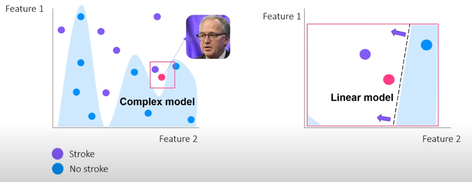
- Explains the local (zoomed-in) approximation for the overall complex model
- Fits a linear model on this zoomed-in portion
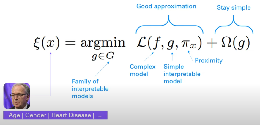
- \(G\) can be collection of interpretable models \(\{\) Linear regression, Decision trees, Log Reg…\(\}\)
- \(\pi_{x}\) represents the locality area around \(x\)
- minimize \(\mathcal{L}(f, g, \pi_{x})\) which measures how bad the simple model \(g\) approximates \(f\) within the area of \(\pi_{x}\)
- minimize \(\Omega(g)\) which is measure of complexity of the interpretable model \(g\) such as (# of parameters in linear regression, depth of decision trees, etc.)
Implementation:
Step 1. Calculate the first loss term \(\mathcal{L}(f, g, \pi_{x})\)
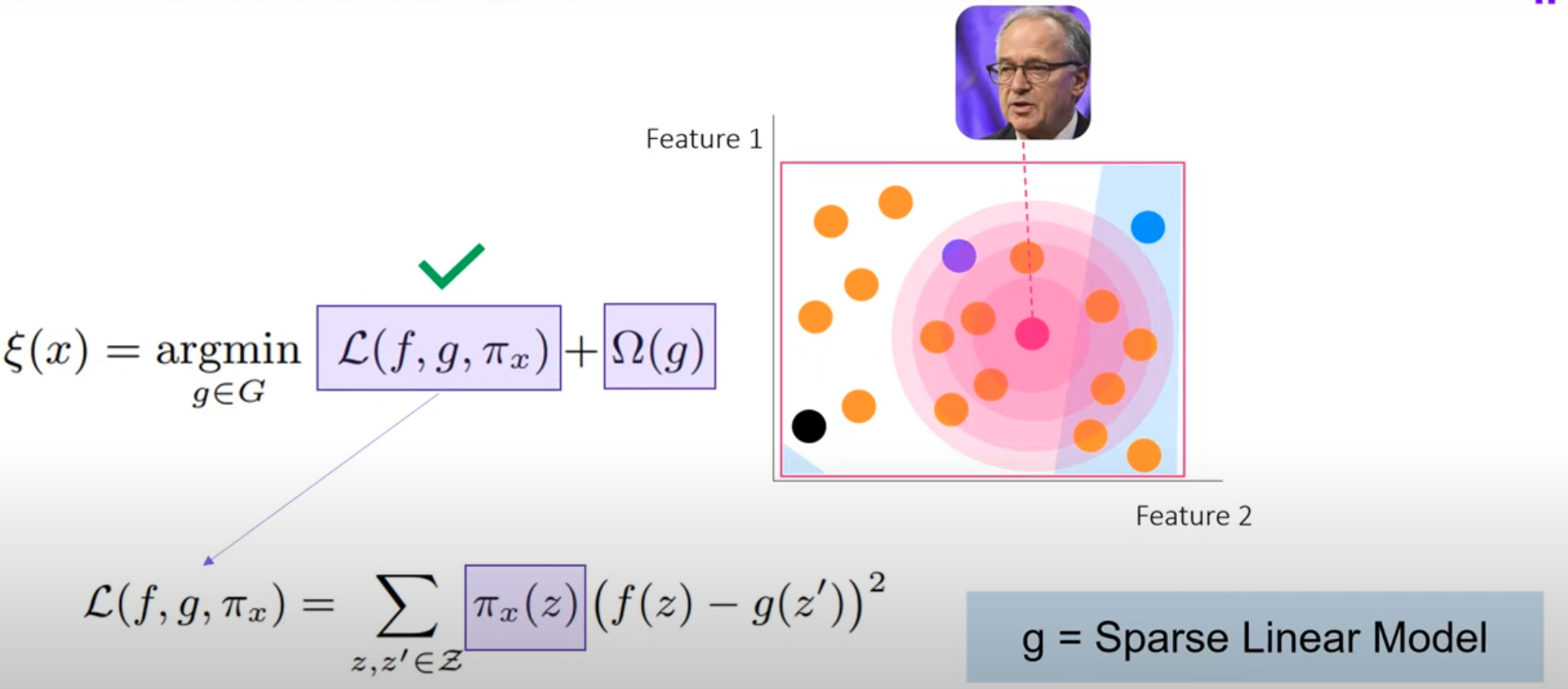
- Within the local area of query point, generate a bunch of random new datapoints
- Classify those datapoints according to the complex model \(f\)
- Use these new data & labels predicted by \(f\) to train a simple model \(g\)
- Loss is then defined as the total deviation from complex model \(f\) to simple model \(g\) for each random generated datapoint
- Additionally, we should weight the errors based on distance from the query point
Step 2. Calculate the second loss term \(\Omega(g)\)
- Ensures the model is as simple as possible
- So you can use something like lasso or ridge regression in a linear model
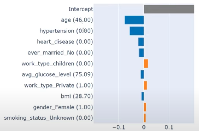
Summary: LIME allows you to see which input features are most relevant for an output prediction, even if the model is black box
2. SHAP (Shapley Additive Explanations)
- Shapley values tells us the weighted average of a features contribution to the output
- Find marginal contributions of each subset of features (to account for interactions between features)
- So we need to iterate over all possible combinations of features and then average (total of \(2^{n}\) subsets)
Example: 2 player game
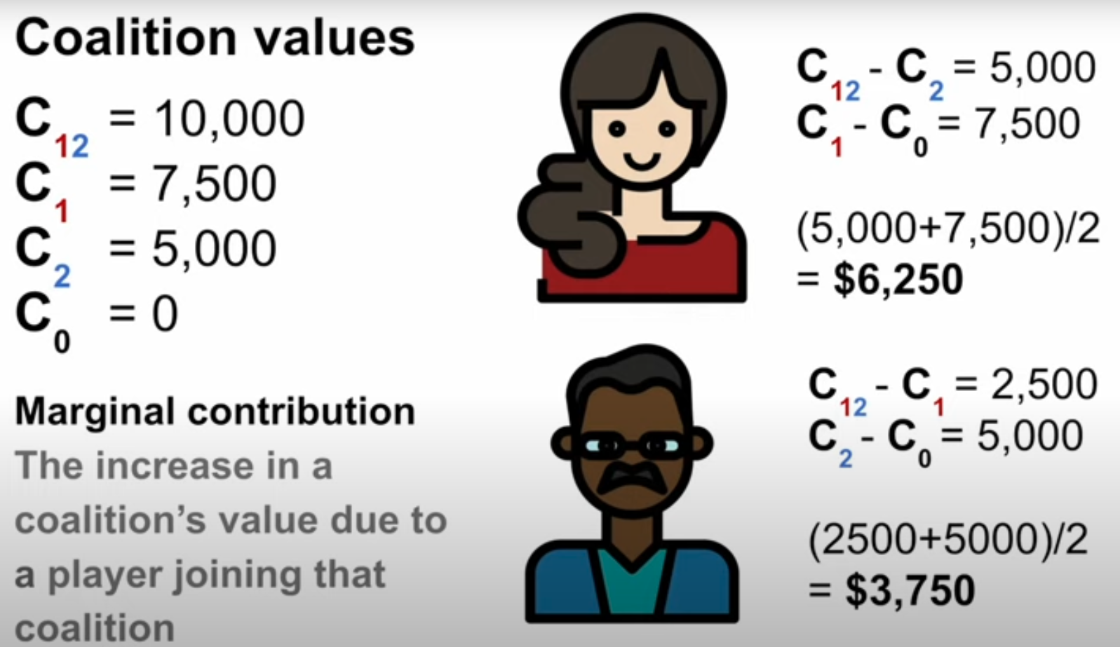
Player 1 and Player 2 work together and generate $10,000
Player 1 alone can generate 7,500
Player 2 alone can generate 5,000
- Shapley(Player 1) = (total - p2 solo contribution) + p1 solo contribution / 2
- Shapley(Player 2) = (total - p1 solo contribution) + p2 solo contribution / 2
Example: 3 player game
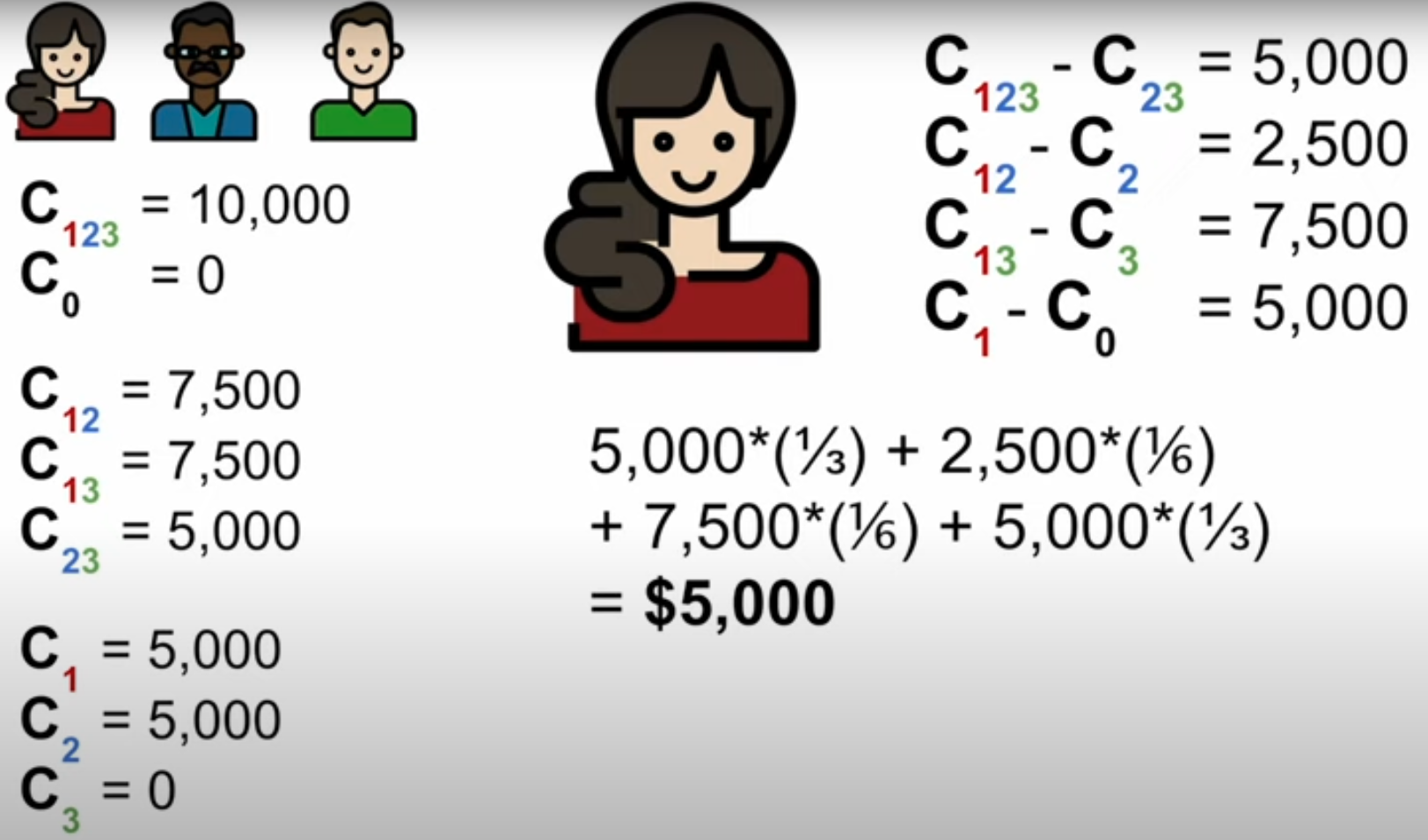
- Shapley(Player 1) = weighted average of all possible subsets that isolate player 1
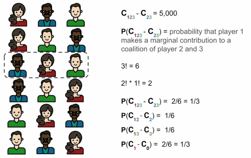
- Weights –> expected marginal contributions
How do we get the weights?
- Weights = number of ways in which Player 1 can join the different coalitions
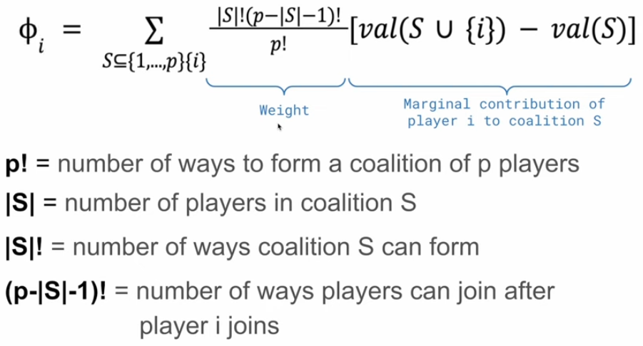
General Shapley Value Formula
3. Counterfactual Explanations
- Person X has a 90% of stroke. If they decrease BMI to 25, then decrease prediction to 30% stroke.
- Counterfactual: The smallest change in input features that changes prediction to another output
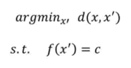
- Find the minimum change from the original input \(x\) to the counterfactual \(x'\) st. the output class is changed \(f(x') = c\)
Generating counterfactuals
- White box approach: if we have access to the model (model-specific)
- Black box approach: if we only have inputs and outputs (model-agnostic)
Output of a counterfactual explainer results in what features need to change by what value in order to output a designated class
4. Causality and Graph Neural Networks
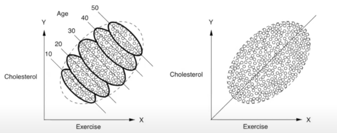
Def: Confounding Factors are variables that influence both independent and dependent variables. The existence of them explains why correlation != causation.
- Let X be an ind. variable and Y be a dep variable. We say that X and Y are confounded by Z if Z causally influences both X and Y.
- Ex: Suppose we want to see if carb intake (X) affects cholesterol levels (Y). A confounding variable (Z) could be exercise level, as people who exercise more can eat more carbs and also impact cholesterol.
Goal: Isolate causal effects by reducing confounding factors by blocking paths (do-calculus)
Pearls Causal Hierarchy and Do-Calculus
- Association (Seeing Patterns): Provides observational info and correlations
- Ex: Observing students who study more get higher test scores
- Interventions (Doing Something): Approximating what happens if you change something and the effects of actions
- Ex: Making people study more to observe the effect on scores
- Counterfactuals (Imagining What-Ifs): Imagining hypotheticals about what happens after-the-fact
- Ex: Imagining what would happen if people did not study at all
Neural Causal Models
- Goal is to approximate connections between variables by learning associational/interventional/counterfactual distributions
5. Bayesian Networks
A Bayesian Network is a directed acyclical graph (DAG) with nodes and directed links that explains the probabilistic relationships (and influences) between variables:
- Node = feature (or multiple features)
- Link = indicates one node directly influences another
Distributions:
- Each node (which represents features e.g., age, height, bmi) is assigned a distribution
- Give node X, a bayesian network requires a distribution \(P(X \mid parent(X))\) where parent(X) indicates the parent nodes of X
- If X has no parents, then the distribution is just P(X) aka the “prior”
How Are Distributions Assigned?
- Learned from data
- Experts specified
- Hybrid
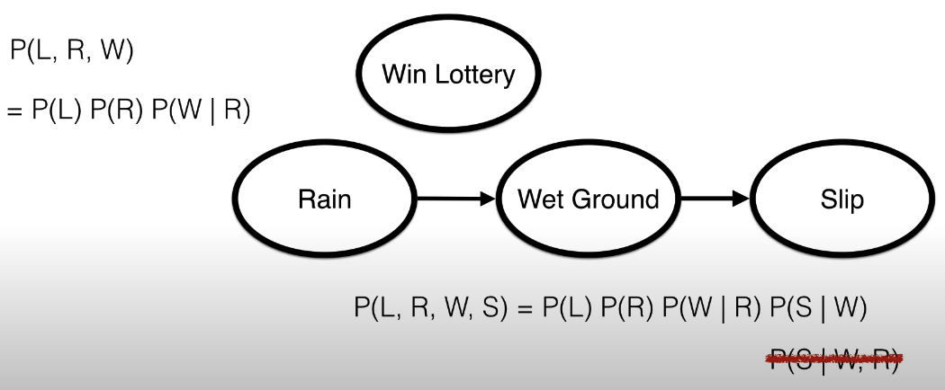
- Notice how we don’t factor in the rain when calculating probability of slipping. All we care about is that the ground is wet.
Inference: Given a Bayesian Network describing P(X,Y,Z), what is P(Y)
- Enumeration (brute force)